Bayesian Network : A statistical Model 

Introduction

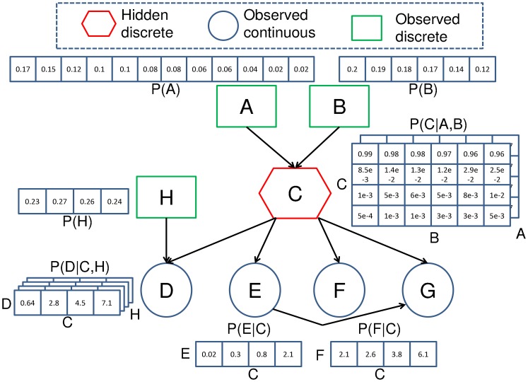
A Bayesian network is a probabilistic graphical model which represents a set of variables and their conditional dependencies using a DAG (directed acyclic graph).

Bayes Network, decision network, or belief network are alternate name for bayesian network.

Bayesian Networks are probabilistic, on the grounds that these networks are worked from a likelihood dispersion(probability distribution), and furthermore use probability theory for forecast and anomaly detection. 

This type of Probabilistic Graphical Model  can be used to build models from data and/or expert opinion.

This specific idea of Bayesian Neural Networks comes to play when unseen data which is creating uncertainty  is fed into the neural network.

The proportion of this uncertainty in the forecast, which is absent from the Neural Network Architectures, is the thing that Bayesian Neural Nets clarifies. It can tackle overfitting and obviously aids in estimating uncertainty and probability distributions.

How Bayesian Network functions?

Bayesian Neural Network alludes to the expansion of the standard network concerning the past inference.

Bayesian Network’s super power

Whenever uncertainty is high, outright and absolute, Bayesian Neural Networks ends up being extremely effective and viable in explicit settings.

A deep neural network could perform exceptionally well with the non linear data and can formulated logical inference with the data even without historical experience with the same data but at the same time the data requirement will be too much for the training purpose and overfitting might surface. 

The scrape which arises in the current circumstance is that the neural nets, as seen previously functions exceptionally well with the data which is fed for the training purpose only but fail to meet expectations when new and unfamiliar foreign data is fed into the neural framework. This prompts the Nets being heedless to specific uncertainties in the training data itself, driving them to be overconfident about the forecasting which could be misdirecting.

To get rid of mistakes, for example, these, the Bayesian Neural Networks are thusly utilised.

The principle item and thought behind the Bayesian Neural Networks are that each unit is in relationship with the probability distribution, which incorporates the loads(weights) and the biases. These arbitrary factors are known as the random variables , which will offer a totally different value at each time when it is accessed.

For an instance, 

Let ‘X’ be a random variable representing normal distribution. 

Every time X is accessed, a dissimilar estimation(divergent) X is calculated. And this process is called Sampling.  Also the derived value from each sample is probability distribution dependent.

What does a Bayesian networks predict?

These networks  can be used for a wide range of tasks including prediction, anomaly detection, diagnostics, automated insight, reasoning, time series prediction and decision making under uncertainty.

Bayesian networks can also be used to predict the joint probability over multiple outputs (discrete and or continuous). This is useful when it is not enough to predict two variables separately, whether using separate models or even when they are in the same model.

USE OF POMEGRANATE LIBRARY

Pomegranate is a Python bundle that executes quick and adaptable probabilistic models going from singular likelihood circulations to compositional models, for example, Bayesian organizations and covered up Markov models. The center way of thinking behind pomegranate is that all probabilistic models can be seen as a likelihood dissemination in that they all yield likelihood gauges for tests and can be refreshed given examples and their related loads. The essential outcome of this view is that the parts that are carried out in pomegranate can be stacked more deftly than different bundles. For instance, one can assemble a Gaussian combination model simply as building a dramatic or log ordinary blend model. In any case, that is not all! One can make a Bayes classifier that utilizes various sorts of appropriations on each highlights, maybe displaying time-related highlights utilizing a remarkable conveyance and tallies utilizing a Poisson circulation. Ultimately, since these compositional models themselves can be seen as likelihood appropriations, one can construct a combination of Bayesian organizations or a secret Markov model Bayes' classifier that makes expectations over groupings.

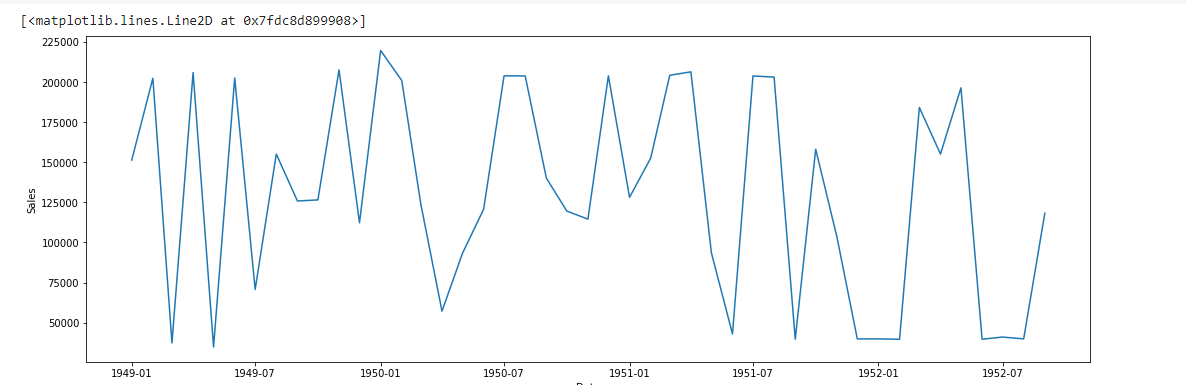
The dataset we are using here looks somewhat like :

GRAPH BETWEEN MONTH AND SALES & CHECK THE STATIONARITY

STATIONARITY : Time Series has a particular behaviour over time, there is a very high probability that it will follow the same in the future.

HOW TO REMOVE STATIONARITY?

• Constant Mean
• Constant Variance
• Autocovariance that doesn't depend on time

This Graph is not Stationarity

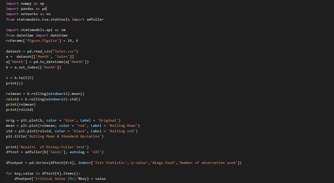
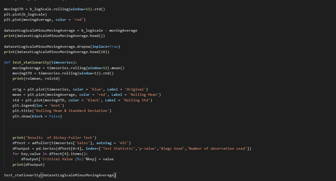
TEST TO CHECK STATIONARITY

1. Rolling Statistic : Plot the moving average or moving variance and see if it varies with time. More of a visual technique

2. Dickey-Fuller Test : Null hypothesis is that the Time Series is non-stationary the test result comprise of a Test Statistic and some Critical Value.

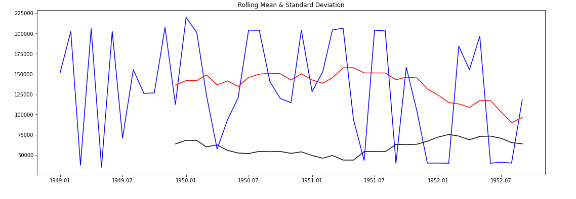
ROLLING MEAN & STANDARD DEVIATION GRAPH

The RED color is Rolling Mean & The BLACK color is Standard Deviation.

Rolling Mean and Standard Deviation both are not constant. That's Means The Data is not Stationarity

DICKEY-FULLER TEST

Statistical tests make strong assumptions about your data. They can only be used to inform the degree to which a null hypothesis can be rejected or fail to be reject. The result must be interpreted for a given problem to be meaningful.

Nevertheless, they can provide a quick check and confirmatory evidence that your time series is stationary or non-stationary.

The Dickey-Fuller test is a type of statistical test called a unit root test.

The intuition behind a unit root test is that it determines how strongly a time series is defined by a trend.

There are a number of unit root tests and the Dickey-Fuller may be one of the more widely used. It uses an autoregressive model and optimizes an information criterion across multiple different lag values.

The null hypothesis of the test is that the time series can be represented by a unit root, that it is not stationary (has some time-dependent structure). The alternate hypothesis (rejecting the null hypothesis) is that the time series is stationary.

Null Hypothesis (H0): If failed to be rejected, it suggests the time series has a unit root, meaning it is non-stationary. It has some time dependent structure.

Alternate Hypothesis (H1): The null hypothesis is rejected; it suggests the time series does not have a unit root, meaning it is stationary. It does not have time-dependent structure. We interpret this result using the p-value from the test. A p-value below a threshold (such as 5% or 1%) suggests we reject the null hypothesis (stationary), otherwise a p-value above the threshold suggests we fail to reject the null hypothesis (non-stationary).

p-value > 0.05: Fail to reject the null hypothesis (H0), the data has a unit root and is non-stationary.

p-value <= 0.05: Reject the null hypothesis (H0), the data does not have a unit root and is stationary. Below is an example of calculating the Dickey-Fuller test on the Daily Female Births dataset. The statsmodels library provides the adfuller() function that implements the test.

P-Values : Another quantitative measure for reporting the result of a test of hypothesis is the p-value. The p-value is the probability of the test statistic being at least as extreme as the one observed given that the null hypothesis is false.

Critical Values : Critical Values for a test of hypothesis depend upon a test statistic, which is specific to the type of test, and the significance level,, α, which defines the sensitivity of the test. A value of α = 0.05 implies that the null hypothesis is rejected 5 % of the time when it is in fact true. The choice of α is somewhat arbitrary, although in practice values of 0.1, 0.05, and 0.01 are common. Critical values are essentially cut-off values that define regions where the test statistic is unlikely to lie

Akaike’s information criterion (AIC) : The Akaike information criterion (AIC) is a mathematical method for evaluating how well a model fits the data it was generated from. In statistics, AIC is used to compare different possible models and determine which one is the best fit for the data.

ROLLING MEAN & STANDARD DEVIATION GRAPH

The RED color is Rolling Mean & The BLACK color is Standard Deviation Rolling Mean and Standard Deviation both are constant. That's Means The Data is Stationarity If p-value is less than 0.5 this mean our dataset is stationarity but Now the P-value is less than 0.5 and tha value is 0.000045. This Mean is, Data Is Stationarity

Exponential Weighting Method

The exponential weighting method has an infinite impulse response. The algorithm computes a set of weights, and applies these weights to the data samples recursively. As the age of the data increases, the magnitude of the weighting factor decreases exponentially and never reaches zero. In other words, the recent data has more influence on the statistic at the current sample than the older data. Due to the infinite impulse response, the algorithm requires fewer coefficients, making it more suitable for embedded applications.

The value of the forgetting factor determines the rate of change of the weighting factors. A forgetting factor of 0.9 gives more weight to the older data than does a forgetting factor of 0.1. To give more weight to the recent data, move the forgetting factor closer to 0. For detecting small shifts in rapidly varying data, a smaller value (below 0.5) is more suitable. A forgetting factor of 1.0 indicates infinite memory. All the previous samples are given an equal weight. The optimal value for the forgetting factor depends on the data stream. For a given data stream, to compute the optimal value for forgetting factor.

We observe that the Time Series is stationary & also the series for moving avg & std. dev. is almost parallel to x-axis thus they also have no trend. Also,

p-value has decreased from 0.022 to 0.005. Test Statistic value is very much closer to the Critical values. Both the points say that our current transformation is better than the previous logarithmic transformation. Even though, we couldn't observe any differences by visually looking at the graphs, the tests confirmed decay to be much better. But lets try one more time & find if an even better solution exists. We will try out the simple time shift technique, which is simply:

Given a set of observation on the time series: x0,x1,x2,x3,....xn The shifted values will be: null,x0,x1,x2,....xn <---- basically all xi's shifted by 1 pos to right

Thus, the time series with time shifted values are: null,(x1−x0),(x2−x1),(x3−x2),(x4−x3),....(xn−xn−1)

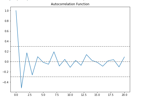
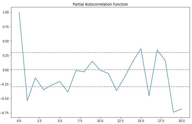
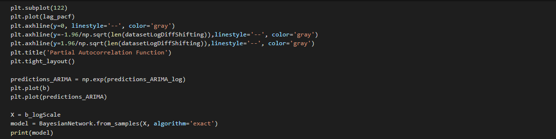
Plotting ACF & PACF

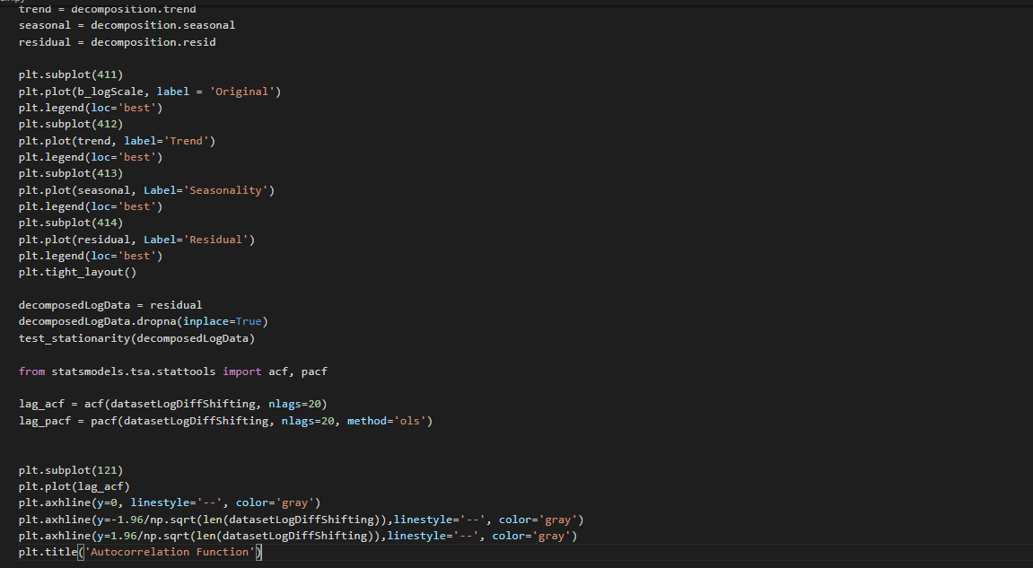
From the ACF graph, we see that curve touches y=0.0 line at x=2. Thus, from theory, Q = 2 From the PACF graph, we see that curve touches y=0.0 line at x=2. Thus, from theory, P = 2

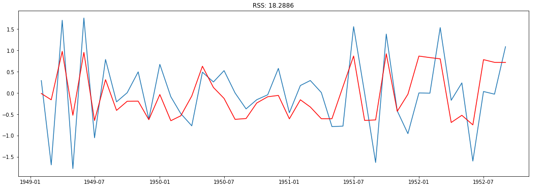
ARIMA is AR + I + MA. Before, we see an ARIMA model, let us check the results of the individual AR & MA model. Note that, these models will give a value of RSS. Lower RSS values indicate a better model.

ARIMA MODEL

ARIMA(Auto Regressive Integrated Moving Average) is a combination of 2 models AR(Auto Regressive) & MA(Moving Average). It has 3 hyperparameters - P(auto regressive lags),d(order of differentiation),Q(moving avg.) which respectively comes from the AR, I & MA components. The AR part is correlation between prev & current time periods. To smooth out the noise, the MA part is used. The I part binds together the AR & MA parts.

ARIMA is AR + I + MA. Before, we see an ARIMA model, let us check the results of the individual AR & MA model. Note that, these models will give a value of RSS. Lower RSS values indicate a better model.

Disp=-1 is a parameter

disp int, optional If True, convergence information is printed. For the default l_bfgs_b solver, disp controls the frequency of the output during the iterations. disp < 0 means no output in this case.

Cumulative Sum (CUSUM) : control chart of autoregressive integrated moving average ARIMA(p,d,q) process observations with exponential white noise. The explicit formula are derived and the numerical integrations algorithm is developed for comparing the accuracy. We derived the explicit formula for ARL by using the Integral equations (IE) which is based on Fredholm integral equation. Then we proof the existence and uniqueness of the solution by using the Banach’s fixed point theorem. For comparing the accuracy of the explicit formulas, the numerical integration (NI) is given by using the Gauss-Legendre quadrature rule. Finally, we compare numerical results obtained from the explicit formula for the ARL of ARIMA(1,1,1) processes with results obtained from NI. The results show that the ARL from explicit formula is close to the numerical integration with an absolute percentage difference less than 0.3% with m = 800 nodes. In addition, the computational time of the explicit formula are efficiently smaller compared with NI.

Predictions

AR.plot Graph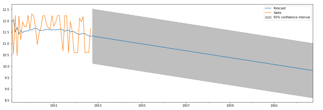

‘The Bayesian Neural Networks, hence, conveniently deal with the issue of uncertainties in the training data which is so fed.’

- Team Ezapp