
Customer Churn Prediction
Python is one of the most frequently used programming languages for financial data analysis, with a lot of helpful libraries and implicit usefulness. In this blog, you'll perceive how Python's machine learning libraries can be utilized for customer churn prediction.
INTRODUCTION TO CUSTOMER CHURN PREDICTION
Customer churn is a financial term that refers to the loss of a client or customer—that is, when a customer ceases to interact with a company or business. Also, the churn rate is the rate at which clients or customers are leaving an company inside a particular timeframe. An churn rate higher than a specific threshold can have both substantial and theoretical impacts on an companie's business achievement. In a perfect world, companies like to hold however many clients as they can.With the appearance of advanced data science and machine learning techniques, it's presently workable for companies to identify potential customers who may cease doing business with them in the near future. In this article, you'll perceive how a bank can predict customer churn dependent on various client ascribes like age, gender, geography, and more. The details of the features utilized for client stir expectation are given in a later area.
Here's an overview of the steps we'll take in this blog:
- Importing the libraries
- Loading the dataset
- Selecting relevant features
- Converting categorical columns to numeric ones
- Preprocessing the data
- Training a machine learning algorithm
- Evaluating the machine learning algorithm
- Evaluating the dataset features
Step 1: Importing the Libraries
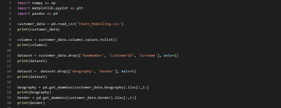
The first step, as always, is to import the required libraries. Execute the following code to do so:
Step 2: Loading the Dataset
The second step is to load the dataset from the local CSV file into your Python program. Let's use the read_csv method of the pandas library. Execute the following code:
Step 3: Feature Selection
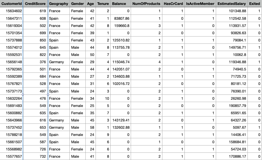
As a reminder, there are 14 columns total in our dataset (see the screenshot above). You can verify this by executing the following code:
Not all columns affect the customer churn. Let's discuss each column one by one:
RowNumber—corresponds to the record (row) number and has no effect on the output. This column will be removed.CustomerId—contains random values and has no effect on customer leaving the bank. This column will be removed.Surname—the surname of a customer has no impact on their decision to leave the bank. This column will be removed.CreditScore—can have an effect on customer churn, since a customer with a higher credit score is less likely to leave the bank.Geography—a customer's location can affect their decision to leave the bank. We'll keep this column.Gender—it's interesting to explore whether gender plays a role in a customer leaving the bank. We'll include this column, too.Age—this is certainly relevant, since older customers are less likely to leave their bank than younger ones.Tenure—refers to the number of years that the customer has been a client of the bank. Normally, older clients are more loyal and less likely to leave a bank.Balance—also a very good indicator of customer churn, as people with a higher balance in their accounts are less likely to leave the bank compared to those with lower balances.NumOfProducts—refers to the number of products that a customer has purchased through the bank.HasCrCard—denotes whether or not a customer has a credit card. This column is also relevant, since people with a credit card are less likely to leave the bank.IsActiveMember—active customers are less likely to leave the bank, so we'll keep this.EstimatedSalary—as with balance, people with lower salaries are more likely to leave the bank compared to those with higher salaries.Exited—whether or not the customer left the bank. This is what we have to predict.
After careful observation of the features, we'll remove the RowNumber, CustomerId, and Surname columns from our feature set. All the remaining columns do contribute to the customer churn in one way or another.
To drop these three columns, execute the following code:
Notice here that we've stored our filtered data in a new data frame named dataset. The customer_data data frame still contains all the columns. We'll reuse that later.
Step 4: Converting Categorical Columns to Numeric Columns
Machine learning algorithms work best with numerical data. However, in our dataset, we have two categorical columns: Geography and Gender. These two columns contain data in textual format; we need to convert them to numeric columns.
Let's first isolate these two columns from our dataset. Execute the following code to do
One way to convert categorical columns to numeric columns is to replace each category with a number. For instance, in the Gender column, female can be replaced with 0 and male with 1, or vice versa. This works for columns with only two categories.
For a column like Geography with three or more categories, you can use the values 0, 1, and 2 for the three countries of France, Germany, and Spain. However, if you do this, the machine learning algorithms will assume that there is an ordinal relationship between the three countries. In other words, the algorithm will assume that 2 is greater than 1 and 0, which actually is not the case in terms of the underlying countries the numbers represent.
A better way to convert such categorical columns to numeric columns is by using one-hot encoding. In this process, we take our categories (France, Germany, Spain) and represent them with columns. In each column, we use a 1 to designate that the category exists for the current row, and a 0 otherwise.
In this case, with the three categories of France, Germany, and Spain, we can represent our categorical data with just two columns (Germany and Spain, for example). Why? Well, if for a given row we have that Geography is France, then the Germany and Spain columns will both have a 0, implying that the country must be the remaining one not represented by any column. Notice, then, that we do not actually need a separate column for France.
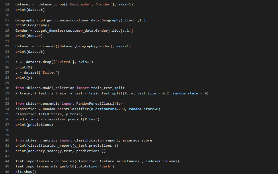
Let's convert both the Geography and Gender columns into numeric columns. Execute the following script:
The get_dummies method of the pandas library converts categorical columns to numeric columns. Then, .iloc[:,1:] ignores the first column and returns the rest of the columns (Germany and Spain). As noted above, this is because we can always represent "n" categories with "n - 1" columns.
Now if you open the Geography and customer_data data frames in the Variable Explorer pane, you should see something like this:
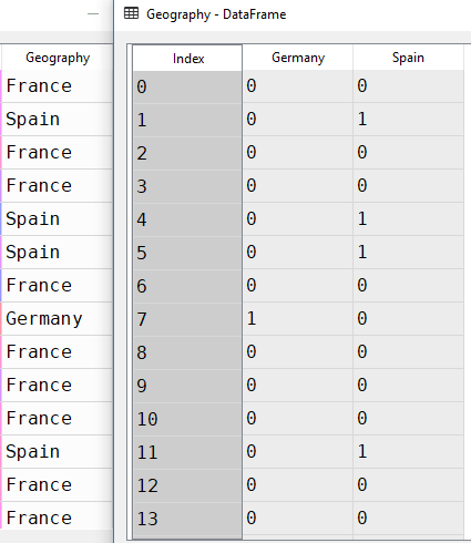
In accordance with our earlier explanation, the Geography data frame contains two columns instead of three. When the geography is France, both Germany and Spain contain 0. When the geography is Spain, you can see a 1 in the Spain column and a 0 in the Germany column. Similarly, in the case of Germany, you can see a 1 in the Germany column and a 0 in the Spain column.
Next, we need to add the Geography and Gender data frames back to the data set to create the final dataset. You can use the concat function from pandas to horizontally concatenate two data frames:
Step 5: Data Preprocessing
Our data is now ready, and we can train our machine learning model. But first, we need to isolate the variable that we're predicting from the dataset.
Here, X is our feature set; it contains all the columns except the one that we have to predict (Exited). The label set, y, contains only the Exited column.
So we can later evaluate the performance of our machine learning model, let's also divide the data into a training and test set. The training set contains the data that will be used to train our machine learning model. The test set will be used to evaluate how good our model is. We'll use 20% of the data for the test set and the remaining 80% for the training set (specified with the test_size argument):
Step 6: Machine Learning Algorithm Training
Now, we'll use a machine learning algorithm that will identify patterns or trends in the training data. This step is known as algorithm training. We'll feed the features and correct output to the algorithm; based on that data, the algorithm will learn to find associations between the features and outputs. After training the algorithm, you'll be able to use it to make predictions on new data.
There are several machine learning algorithms that can be used to make such predictions. However, we'll use the RANDOM FOREST ALGORITHM, since it's simple and one of the most powerful algorithms for classification problems.
To train this algorithm, we call the fit method and pass in the feature set (X) and the corresponding label set (y). You can then use the predict method to make predictions on the test set. Look at the following script:
Step 7: Machine Learning Algorithm Evaluation
Now that the algorithm has been trained, it's time to see how well it performs. For evaluating the performance of a classification algorithm, the most commonly used metrics are the F1 MEASURE PRECISION, RECALL AND ACCURACY. In Python's scikit-learn library, you can use built-in functions to find all of these values.
The results indicate an accuracy of 86.35%, which means that our algorithm successfully predicts customer churn 86.35% of the time. That's pretty impressive for a first attempt!
Step 8: Feature Evaluation
As a final step, let's see which features play the most important role in the identification of customer churn. Luckily, RandomForestClassifier contains an attribute named feature_importance that contains information about the most important features for a given classification.
The following code creates a bar plot of the top 10 features for predicting customer churn:
Final Thoughts
Customer churn prediction is crucial to the long-term financial stability of a company. In this article, you successfully created a machine learning model that's able to predict customer churn with an accuracy of 86.35%. You can see how easy and straightforward it is to create a machine learning model for classification tasks.